From TDA to computational brain modelling:
the case studies of grid cells and epilepsy
XIMENA FERNANDEZ
Durham University
UK Centre for Topological Data Analysis
Brain Modelling Seminar - Oxford University
Topological Data Analysis
Topological inference
Let $X$ be a topological space and let $\mathbb{X}_n = \{x_1,...,x_n\}$ be a finite sample of $X$.
Q: How to infer topological properties of $X$ from $\mathbb{X}_n$?
Topological inference
Let $X$ be a topological space and let $\mathbb{X}_n = \{x_1,...,x_n\}$ be a finite sample of $X$.
Q: How to infer topological properties of $X$ from $\mathbb{X}_n$?
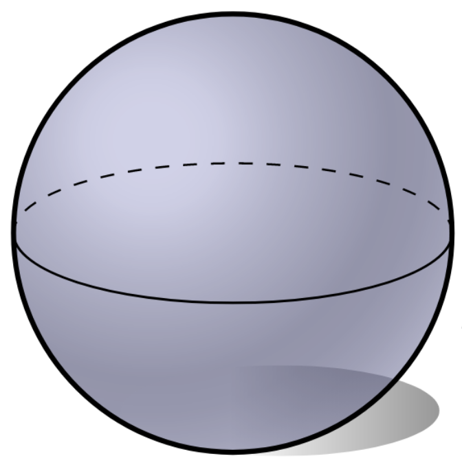
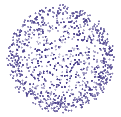
Point cloud
$\mathbb{X}_n \subset \mathbb{R}^D$

For $\epsilon>0$, the $\epsilon$-thickening of $\mathbb{X}_n$:
\[\displaystyle U_\epsilon = \bigcup_{x\in \mathbb{X}_n}B_{\epsilon}(x)\] 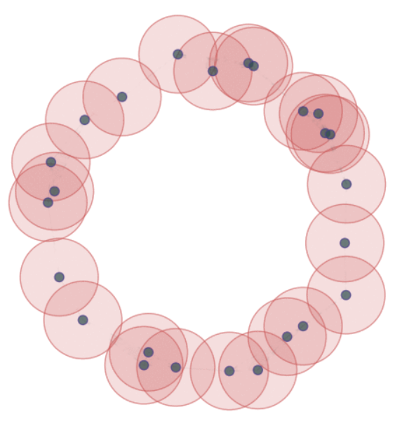
Theorem (Niyogi, Smale & Weinberger, 2008). Given $\mathcal{M}$ a compact submanifold of $\mathbb{R}^D$ of dimension $k$ and $\mathbb{X}_n$ a set of i.i.d. $n$ points drawn according to the uniform probability measure on $\mathcal{M}$, then $$ U_\epsilon \simeq \mathcal{M}$$ with probability $>1-\delta$ if $0<\epsilon< \frac{\tau_\mathcal{M}}{2}$ and $n> \beta_1 \left(\log(\beta_2)+\log\left(\frac{1}{\delta}\right)\right)$.*
*Here $\beta_1=\frac{\mathrm{vol}(\mathcal{M})}{cos^k(\theta_1) \mathrm{vol(B^k_{\epsilon/4})}}$, $\beta_2=\frac{\mathrm{vol}(\mathcal{M})}{\cos^k(\theta_2)\mathrm{vol}(B^k_{\epsilon/8})}$ and $\theta_1=\arcsin\left(\frac{\epsilon}{8\tau_\mathcal M}\right),$ $\theta_2=\arcsin\left(\frac{\epsilon}{16\tau_\mathcal M}\right)$.
Topological inference
Let $X$ be a topological space and let $\mathbb{X}_n = \{x_1,...,x_n\}$ be a finite sample of $X$.
Q: How to infer topological properties of $X$ from $\mathbb{X}_n$?
Point cloud
$\mathbb{X}_n \subset \mathbb{R}^D$
Evolving thickenings

Topological inference
Let $X$ be a topological space and let $\mathbb{X}_n = \{x_1,...,x_n\}$ be a finite sample of $X$.
Q: How to infer topological properties of $X$ from $\mathbb{X}_n$?
Point cloud
$\mathbb{X}_n \subset \mathbb{R}^D$
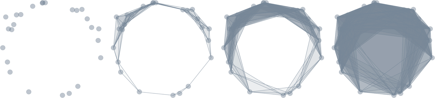
Evolving thickenings
Filtration of simplicial complexes
Topological inference
Let $X$ be a topological space and let $\mathbb{X}_n = \{x_1,...,x_n\}$ be a finite sample of $X$.
Q: How to infer topological properties of $X$ from $\mathbb{X}_n$?
Point cloud
$\mathbb{X}_n \subset \mathbb{R}^D$
Filtration of simplicial complexes
Persistence diagram

Topology of grid cells
Grid cells
- Part of the neural representation of the spatial coordinate system.
- Placed in the medial entorhinal cortex (mEC).
- Discovered by Edvard and May-Britt Moser in 2005.
T. Hafting, M. Fyhn, S, Molden, M.B. Moser, E.I. Moser. Microstructure of a spatial map in the entorhinal cortex. Nature. 2005 Aug; 436(7052) 801-806. - Awarded with Nobel Prize in Physiology or Medicine 2014.

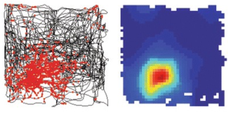
Place cells
- Cognitive representation of a specific location in space.
- Placed in the hippocampus.
- Discovered by John O'Keefe in 1971.
J. O'Keefe, J. Dostrovsky, The hippocampus as a spatial map. Preliminary evidence from unit activity in the freely-moving rat. Brain Research, Volume 34, Issue 1, 1971, 171-175. - Awarded with Nobel Prize in Physiology or Medicine 2014.
A physical model for grid cells activity
The Emergence of Grid Cells: Intelligent Design or Just Adaptation?
Emilio Kropff and Alessandro Treves. Hippocampus (2008)
A physical model for grid cells activity
The Emergence of Grid Cells: Intelligent Design or Just Adaptation?
Emilio Kropff and Alessandro Treves. Hippocampus (2008)
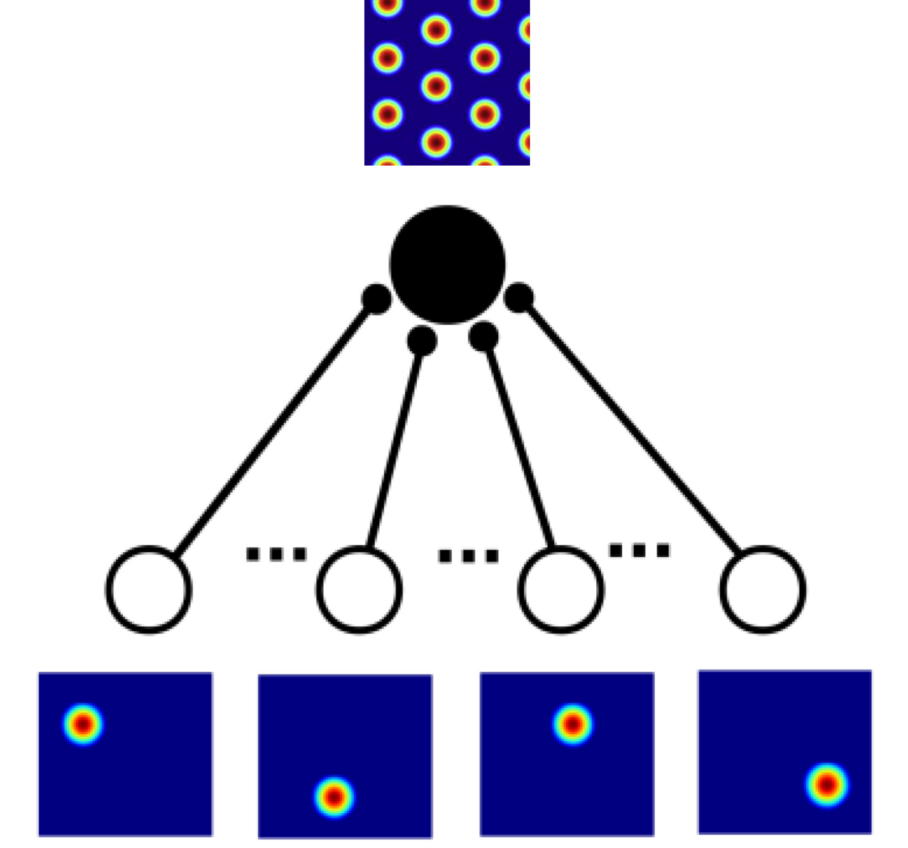
Feedforward network dynamics.
- Input layer: $N_{hip}$ neurons from hippocampus (place cells).
- mEC layer: $N_{mEC}$ neurons from mEC (grid cells).
- Architecture:
- Feed-forward connections between input layer and mEC layer.
- Internal connections between grid-cells.
A physical model for grid cells activity
The total field received by grid cell $i$ at time $t$ is \[h_i(t) = \sum_{j=1}^{N_{I}}W^I_{ij}(t)r_j^I(t) + \sum_{k=1}^{N_{EC}}W^{EC}_{ik}r_k^{EC}(t) \]
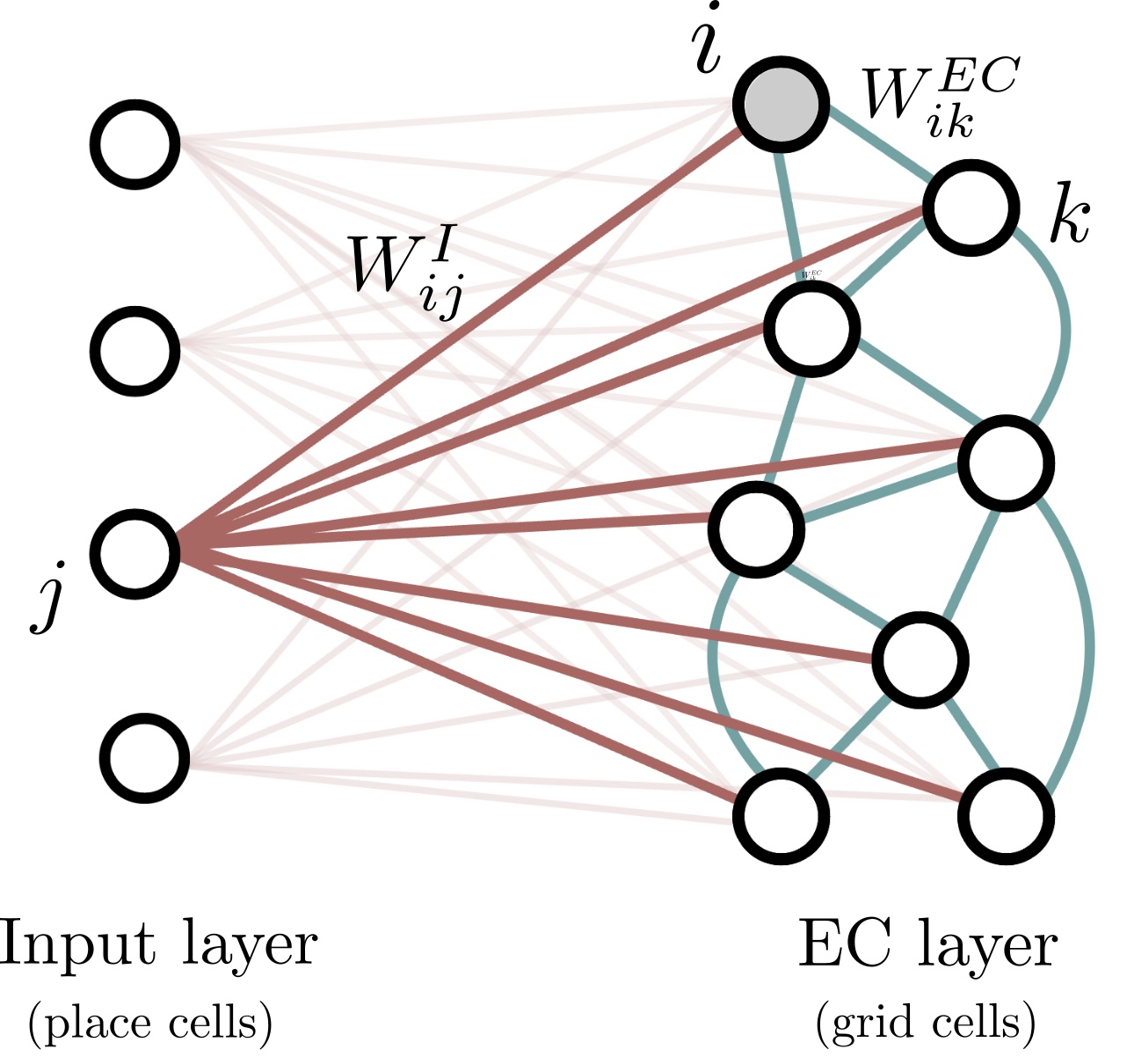
- $W^I_{ij}$ is the weight of the synapse going from neuron $j$ in the input layer to neuron $i$ in the mEC layer.
- $r_j^I(x)$ is the firing rate of the place cell $j$ at time $t$.
- $W^{EC}_{ik}$ is the recurrent excitatory connectivity from neuron $k$ to neuron $i$ in the mEC layer.
- $r_k^{EC}(t)$ is the firing rate of the grid cell $k$ at time $t$.
A physical model for grid cells activity
The total field received by grid cell $i$ at time $t$ is \[h_i(t) = \sum_{j=1}^{N_{I}}W^I_{ij}(t)r_j^I(t) + \sum_{k=1}^{N_{EC}}W^{EC}_{ik}r_k^{EC}(t) \]
- $W^I_{ij}$ is the weight of the synapse going from neuron $j$ in the input layer to neuron $i$ in the mEC layer.
- $r_j^I(x)$ is the firing rate of the place cell $j$ at time $t$.
- $W^{EC}_{ik}$ is the recurrent excitatory connectivity from neuron $k$ to neuron $i$ in the mEC layer.
- $r_k^{EC}(t)$ is the firing rate of the grid cell $k$ at time $t$.
It is updated according to the Hebbian learning rule \[W_{ij}^I(t+1) = W_{ij}^I(t) + \epsilon \left( r_j^I(t)r_i^{EC}(t)-\overline{r_j^I}(t)\overline{r_i^{EC}}(t)\right)\] where $\epsilon$ is a learning parameter and $\overline{\bullet}(t)$ means the exponential moving average at time $t$.
A physical model for grid cells activity
The total field received by grid cell $i$ at time $t$ is \[h_i(t) = \sum_{j=1}^{N_{I}}W^I_{ij}(t)r_j^I(t) + \sum_{k=1}^{N_{EC}}W^{EC}_{ik}r_k^{EC}(t) \]
- $W^I_{ij}$ is the weight of the synapse going from neuron $j$ in the input layer to neuron $i$ in the mEC layer.
- $r_j^I(x)$ is the firing rate of the place cell $j$ at time $t$.
- $W^{EC}_{ik}$ is the recurrent excitatory connectivity from neuron $k$ to neuron $i$ in the mEC layer.
- $r_k^{EC}(t)$ is the firing rate of the grid cell $k$ at time $t$.
It is determined by the position of the individual in the space.
A physical model for grid cells activity
The total field received by grid cell $i$ at time $t$ is \[h_i(t) = \sum_{j=1}^{N_{I}}W^I_{ij}(t)r_j^I(t) + \sum_{k=1}^{N_{EC}}W^{EC}_{ik}r_k^{EC}(t) \]
- $W^I_{ij}$ is the weight of the synapse going from neuron $j$ in the input layer to neuron $i$ in the mEC layer.
- $r_j^I(x)$ is the firing rate of the place cell $j$ at time $t$.
- $W^{EC}_{ik}$ is the recurrent excitatory connectivity from neuron $k$ to neuron $i$ in the mEC layer.
- $r_k^{EC}(t)$ is the firing rate of the grid cell $k$ at time $t$.
It is fixed according to the architecture of the connectivity.
A physical model for grid cells activity
The total field received by grid cell $i$ at time $t$ is \[h_i(t) = \sum_{j=1}^{N_{I}}W^I_{ij}(t)r_j^I(t) + \sum_{k=1}^{N_{EC}}W^{EC}_{ik}r_k^{EC}(t) \]
- $W^I_{ij}$ is the weight of the synapse going from neuron $j$ in the input layer to neuron $i$ in the mEC layer.
- $r_j^I(x)$ is the firing rate of the place cell $j$ at time $t$.
- $W^{EC}_{ik}$ is the recurrent excitatory connectivity from neuron $k$ to neuron $i$ in the mEC layer.
- $r_k^{EC}(t)$ is the firing rate of the grid cell $k$ at time $t$.
It is updated as \[r_i^{EC} (t+1) = G\frac{|h_i^{\mathrm{act}}(t) -T|_{>0}}{{\left(|h_\bullet^{\mathrm{act}}(t)-T|_{>0}\right)}_{\mathrm{avg}}}\] for a gain parameter $G$, a threshold $T$ representing inhibition and internal variables $h_i^{\mathrm{act}}(t)$ and $h_i^{\mathrm{inact}}(t)$ mimicking adaptation or fatigue within the neuron \begin{align*} h_i^{\mathrm{act}}(t+1) &= h_i(t)-h_i^{\mathrm{inact}}(t),\\ h_i^{\mathrm{inact}}(t+1) &= h_i^{\mathrm{inact}} + \beta h_i^{\mathrm{act}}(t)\\ \end{align*} for some parameter $\beta$.
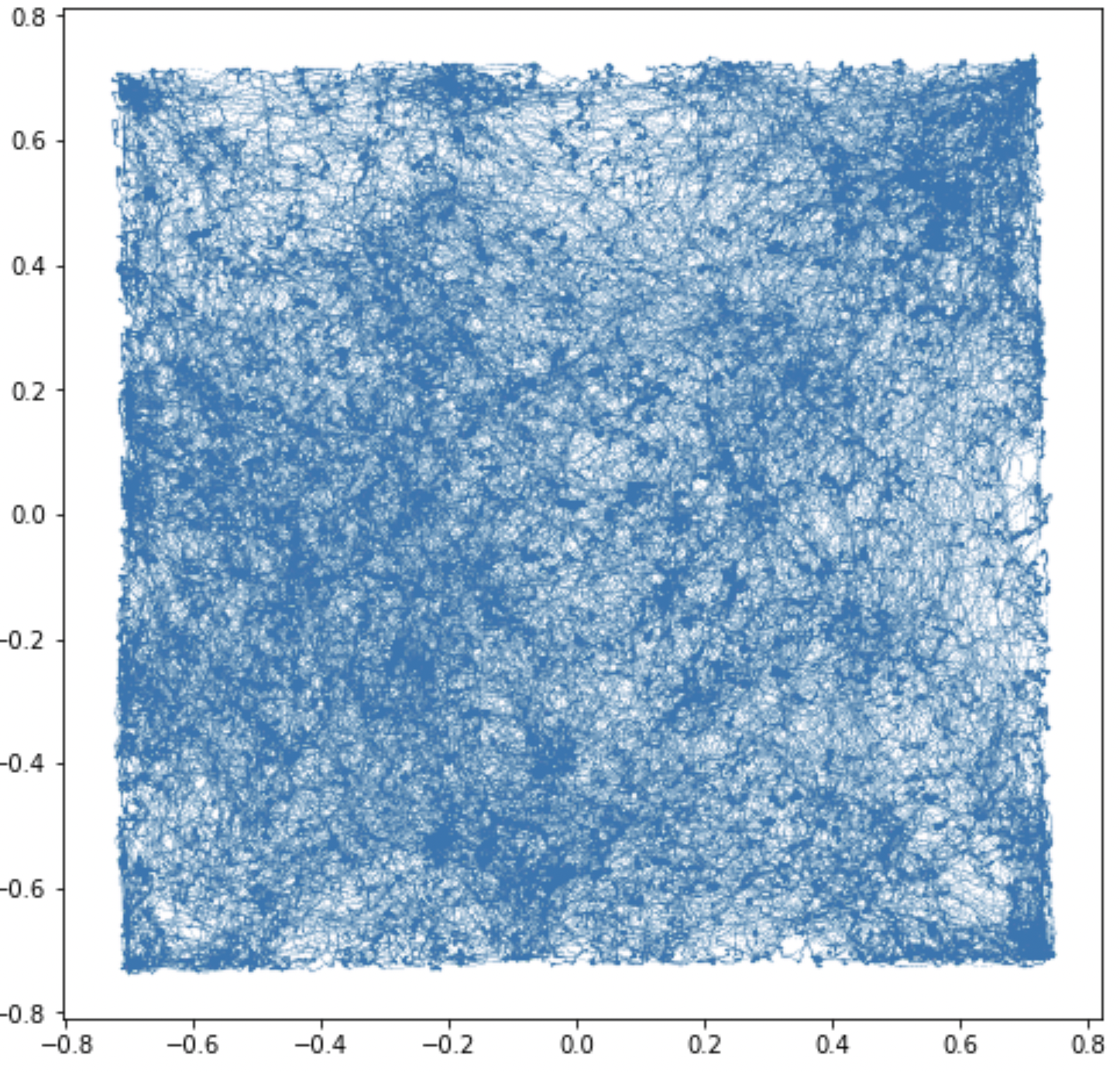
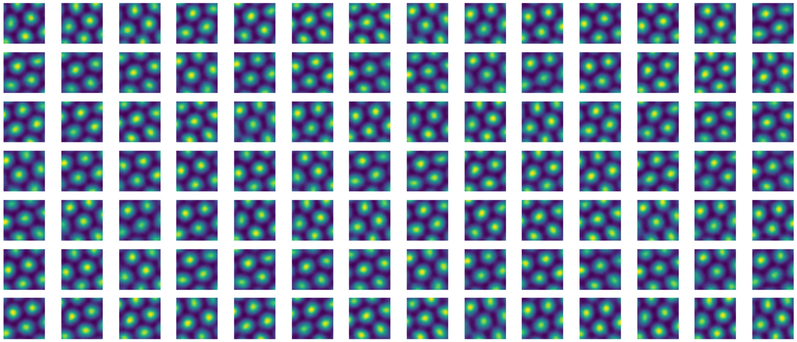
Modelled grid cells
Experiment: Given a square track and a rat moving freely in the environment, we simulated the simultaneous activity of $N_{mEC}$ grid cells at each point $x$ in the arena for a period of time. For a discretization of the environment in $M$ bins and average over time of the spike rate, we obtained a point cloud of $M$ points in $\mathbb R^{N_{mEC}}$.
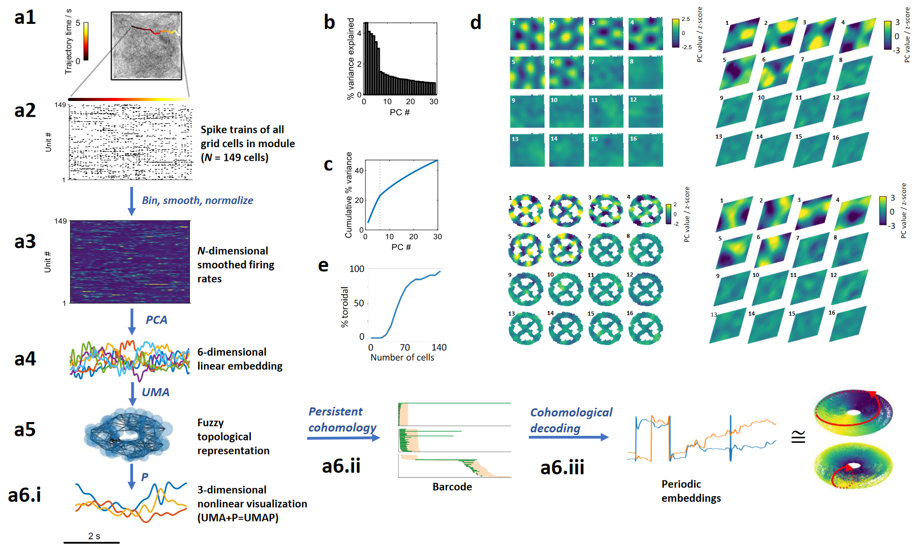
Topology of the attractor
Toroidal topology of population activity in grid cells (2022)
Gardner R, Hermansen E, Pachitariu M, Burak Y, N, Dunn B, Moser M B, Moser E. Nature.
Topology of the attractor
What is the architecture of the
neural network of grid cells?
Modeled grid cells
aligned by a flexible attractor. (2022)
Sabrina Benas, Ximena Fernandez and Emilio Kropff. bioRxiv 2022.06.13.495956.
What is the architecture of the
neural network of grid cells?
2D connectivity

$\bullet$ Gardner R, Hermansen E, Pachitariu M, Burak Y, N, Dunn B, Moser M B, Moser E. Toroidal topology of population activity in grid cells Nature. (2022)
$\bullet$ Guanella A, Kiper D, Verschure P. A model of grid cells based on a twisted torus topology. Int J Neural Syst. 2007 Aug; 17 (4):231-40.
1D connectivity

No connectivity

What is the architecture of the
neural network of grid cells?
Modelled population activity of neurons
2D connectivity

1D connectivity

No connectivity

What is the architecture of the
neural network of grid cells?
Isomap projection of population activity
2D connectivity

1D connectivity

No connectivity

Topology of the attractor
Theorem (Classification of closed surfaces). Let $\mathcal M$ be a compact manifold of dimension 2 without boundary. Let $\chi = b_0-b_1 + b_2$ be the Euler characteristic of $\mathcal M$. There are two cases:
- If $\mathcal M$ is orientable, then it is homeomorphic to a connected sum of $1-\chi/2$ torii.
- If $\mathcal M$ is non-orientable, then it is homeomorphic to a connected sum of $2-\chi$ projective planes.
This result provides a method to univocally determine the homeomorphism type of the geometric structure subjacent in data, provided it is an instance of a closed surface. It is enough to compute (or infer) the following finite list of invariant properties:
- the intrinsic dimension (and prove that it is equal to 2);
- the Euler characteristic (or equivalently, the Betti numbers);
- orientability or non-orientability;
- the (non)existence of singularities and boundary.
Topology of the attractor
Global geometry

a. Smoothed density and Frechet mean across simulations of persistence diagrams with coefficients in $\mathbb{Z}_2$, for 1D (top) and 2D (bottom) connectivity condition. b. As a. but with coefficients in $\mathbb{Z}_3$. c. Distribution of the difference between lifetime of consecutive generators for each simulation (ordered from longest to shortest lifetime) for 1D (left) and 2D (right) connectivity. d. Pie plot and table indicating the number of simulations (out of 100 in each condition) classified according to their Betti numbers.
Topology of the attractor
Local geometry
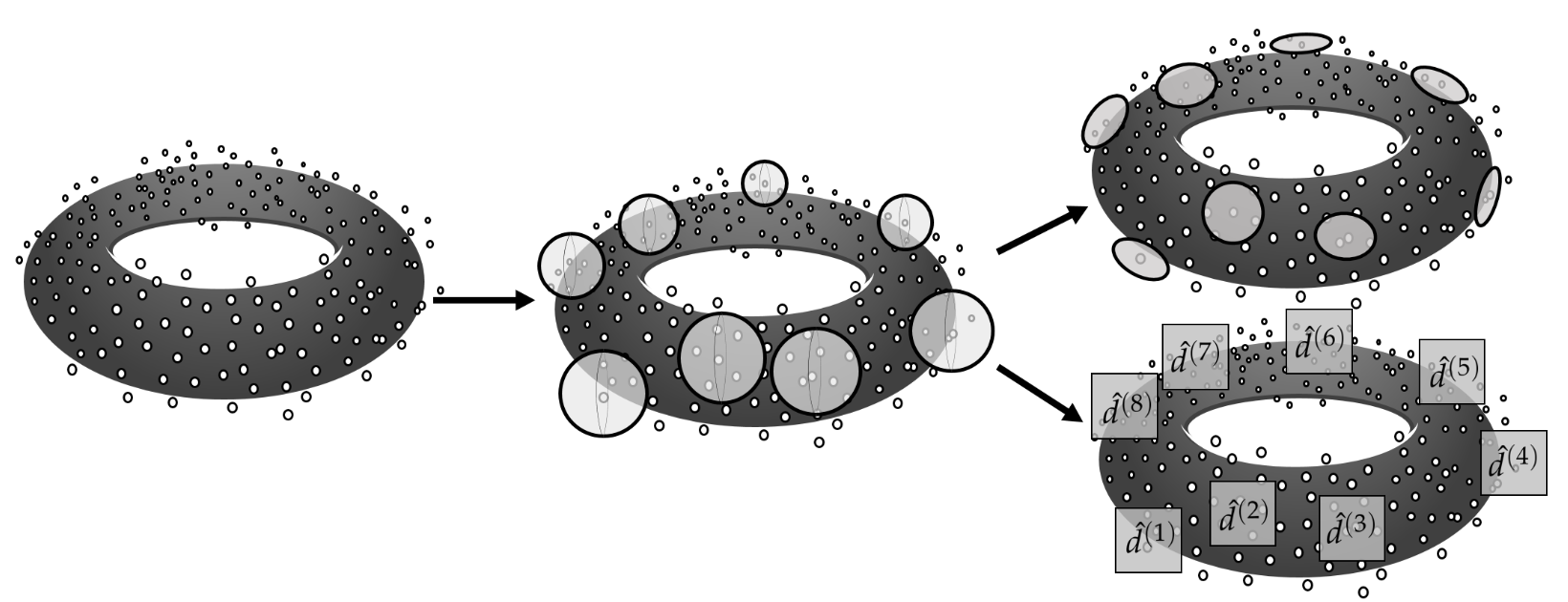 Local homology

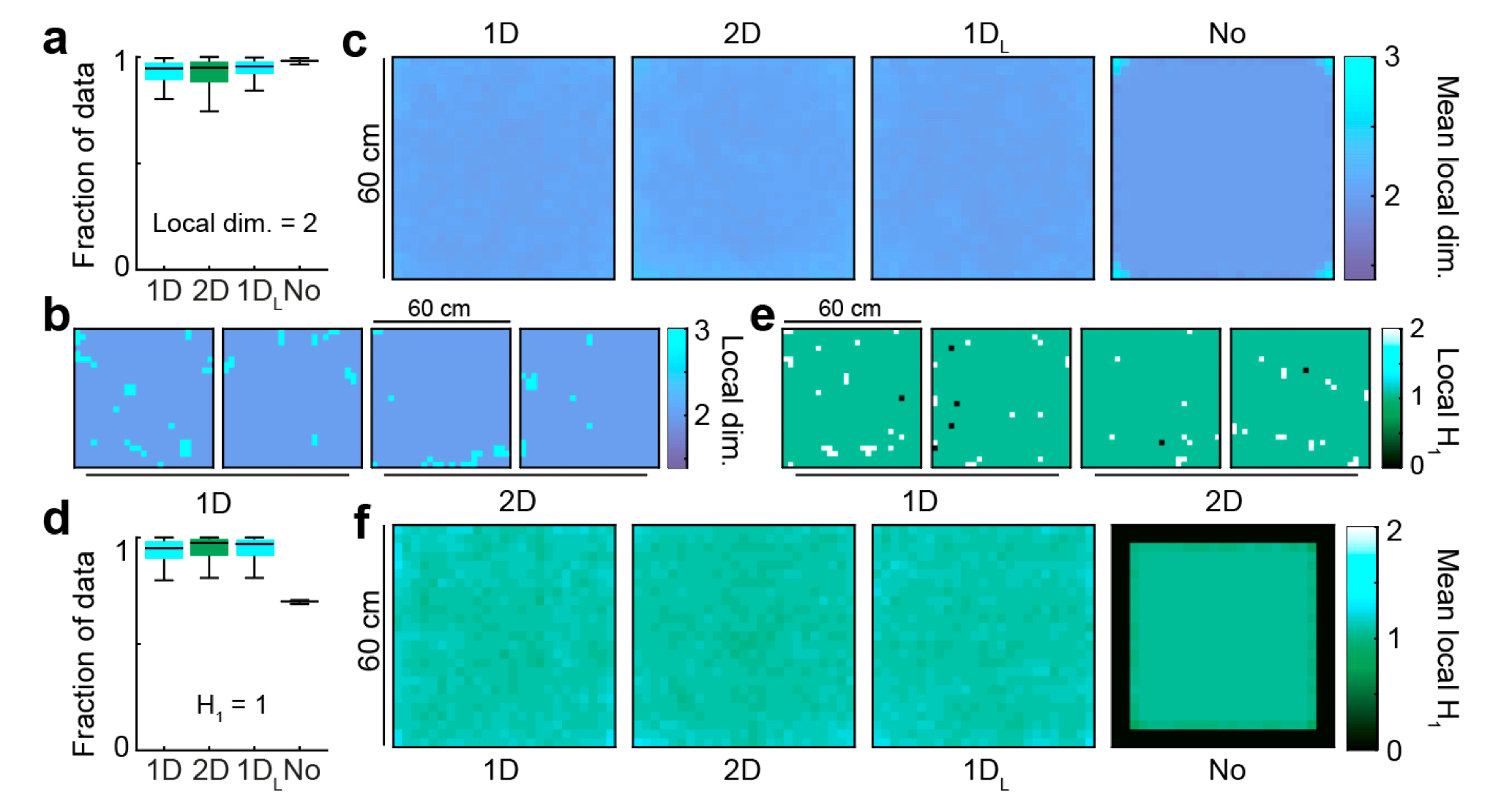
a. Distribution of the fraction of the population data with local dimensionality equal to 2, for every connectivity condition. b. Distribution of local dimensionality across physical space in representative examples of 1D and 2D conditions. c. Average distribution of local dimensionality for all conditions (same color code as in b.) d-f. As a-c but exploring deviations of the local homology $H_1$ from a value equal to 1, the value expected away from boundary points and singularities.
Conclusions
- It is possible (sometimes) to completely determine (infer) the homeomorphism type of a point cloud in high dimensions.
- The population activity of grid cells (and other neurons related to spatial location) has a particular organized geometry that might give information of their self-connectivity in the brain.
- TDA might provide a tool to validate or select physical models (of neural activity).
Topological methods
for detection of epileptic seizures
Topological analysis of EEG/MEG recordings
- Data: Raw multichannel EEG/MEG recordings for different patients during preictal, ictal and interictal states.

Source data: Toronto Western Hospital, Canada. Provided by Diego Mateos.
Topological analysis of EEG/MEG recordings
- Data: Raw multichannel EEG/MEG recordings for different patients during preictal, ictal and interictal states.
- Goal: Detect the epileptic seizure.
Topological analysis of EEG/MEG recordings
Given $X_1, X_2, \dots X_N:[0,T]\to \mathbb{R}$ signals, we construct an embedding in $\mathbb{R}^N$ given by $$\{(X_1(t), X_2(t), \dots, X_N(t)): t\in [0,T]\}$$
Sliding Window Embedding
- Let $X_1, X_2, \dots X_N:[0,T]\to \mathbb{R}$ a set of signals.
- Given a window size $W$, we compute for every $t\in [W,T]$ the embedding of $X_1, X_2, \dots X_N:[t-W, t]\to \mathbb{R}$ in $\mathbb{R}^N$.
Sliding Window Embedding
- Let $X_1, X_2, \dots X_N:[0,T]\to \mathbb{R}$ a set of signals.
- Given a window size $W$, we compute for every $t\in [W,T]$ the embedding of $X_1, X_2, \dots X_N:[t-W, t]\to \mathbb{R}$ in $\mathbb{R}^N$.
Sliding Window Embedding
- Let $X_1, X_2, \dots X_N:[0,T]\to \mathbb{R}$ a set of signals.
- Given a window size $W$, we compute for every $t\in [W,T]$ the embedding of $X_1, X_2, \dots X_N:[t-W, t]\to \mathbb{R}$ in $\mathbb{R}^N$.
- We compute the (persistent) homology of the time evolving sliding window embedding.

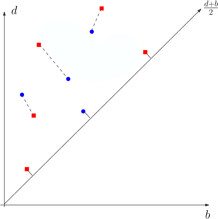
Metric in the space of persistence diagrams
- The Wassertein distance between two diagrams $\mathrm{dgm}_1$ and $\mathrm{dgm}_2$ is \[d_W(\mathrm{dgm}_1, \mathrm{dgm}_2) = \inf_{M \text{ matching}} \left(\sum_{(x,y)\in M} ||x-y||^p\right)^{1/p}\]
Topological analysis of EEG/MEG recordings
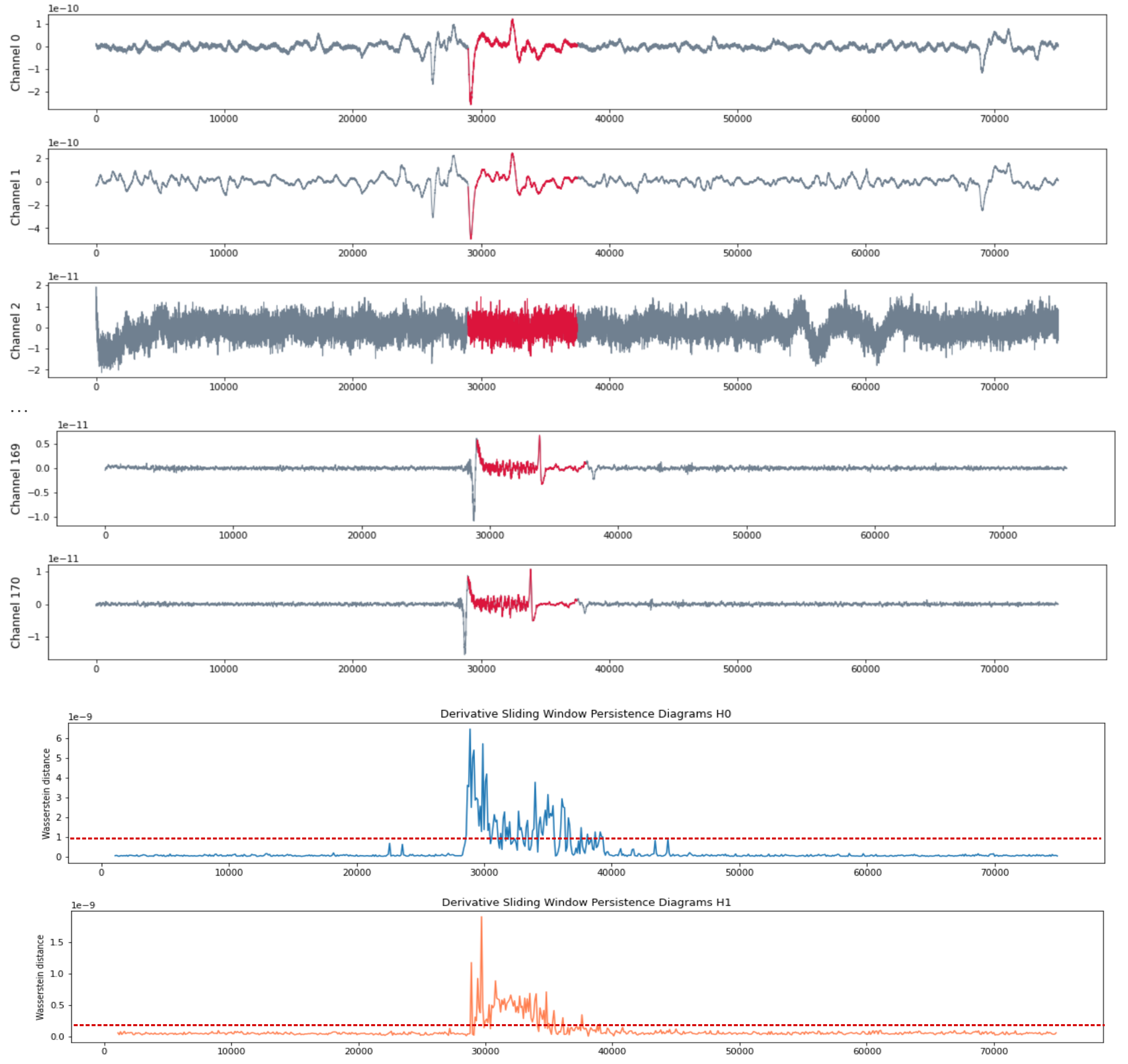
Multichannel signals $\to$ Sliding Window Embedding $\to$ Path of persistent diagrams $\to$ (Estimator of) 1st Derivative
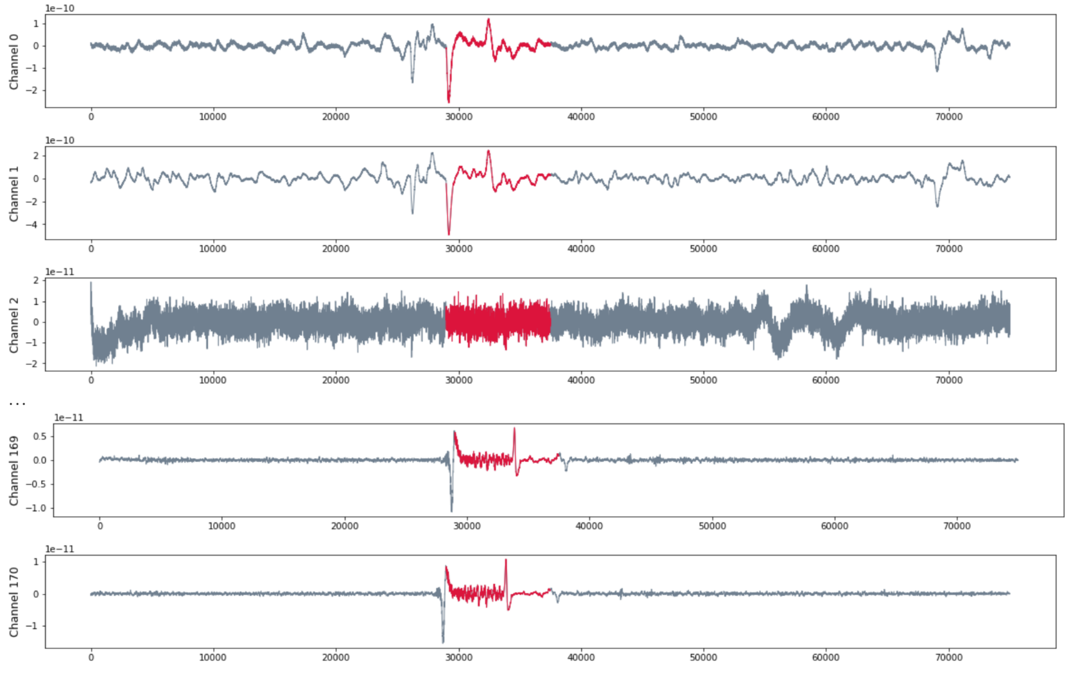
Patient RAO
- MEG with 171 channels
- 120 seg recording with sampling rate 625 HZ

Patient RAO
- MEG with 171 channels
- 120 seg recording with sampling rate 625 HZ
- Seizure starts at $t = 29375$ and ends at $t = 37500$.
Patient RAO
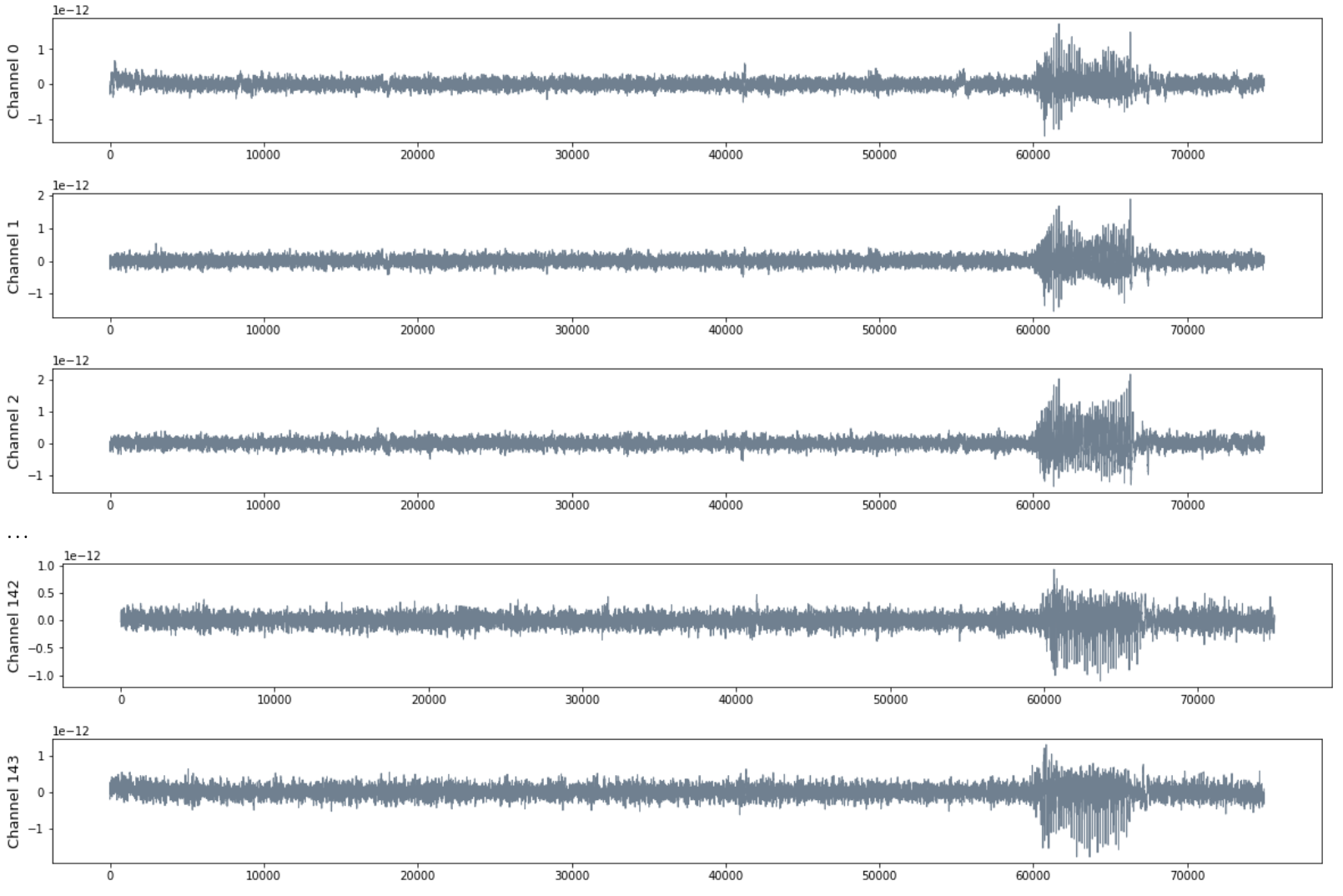
Patient MAC
- MEG with 144 channels
- 120 seg recording with sampling rate 625 HZ
Patient MAC
- MEG with 144 channels
- 120 seg recording with sampling rate 625 HZ
- Seizure starts at $t = 60000$ and ends at $t = 68125$.
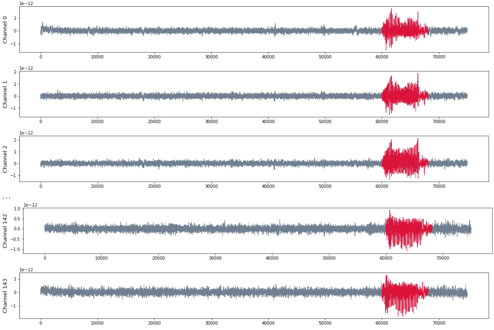
Patient MAC
- MEG with 144 channels
- 120 seg recording with sampling rate 625 HZ
- Seizure starts at $t = 60000$ and ends at $t = 68125$.

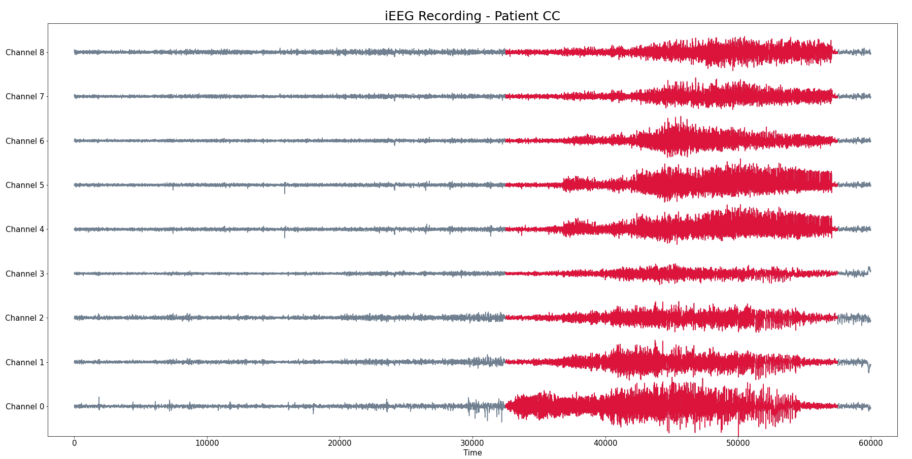
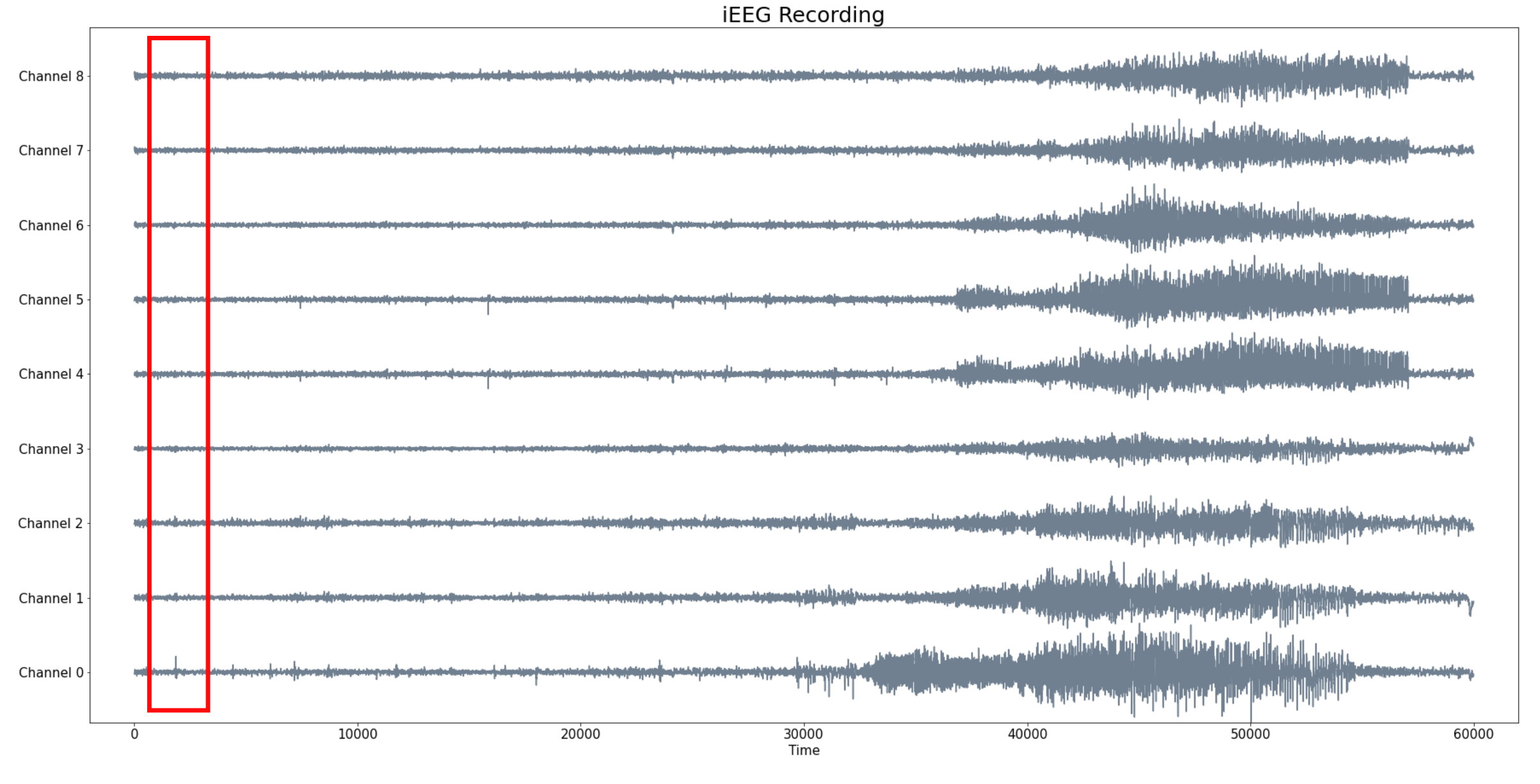
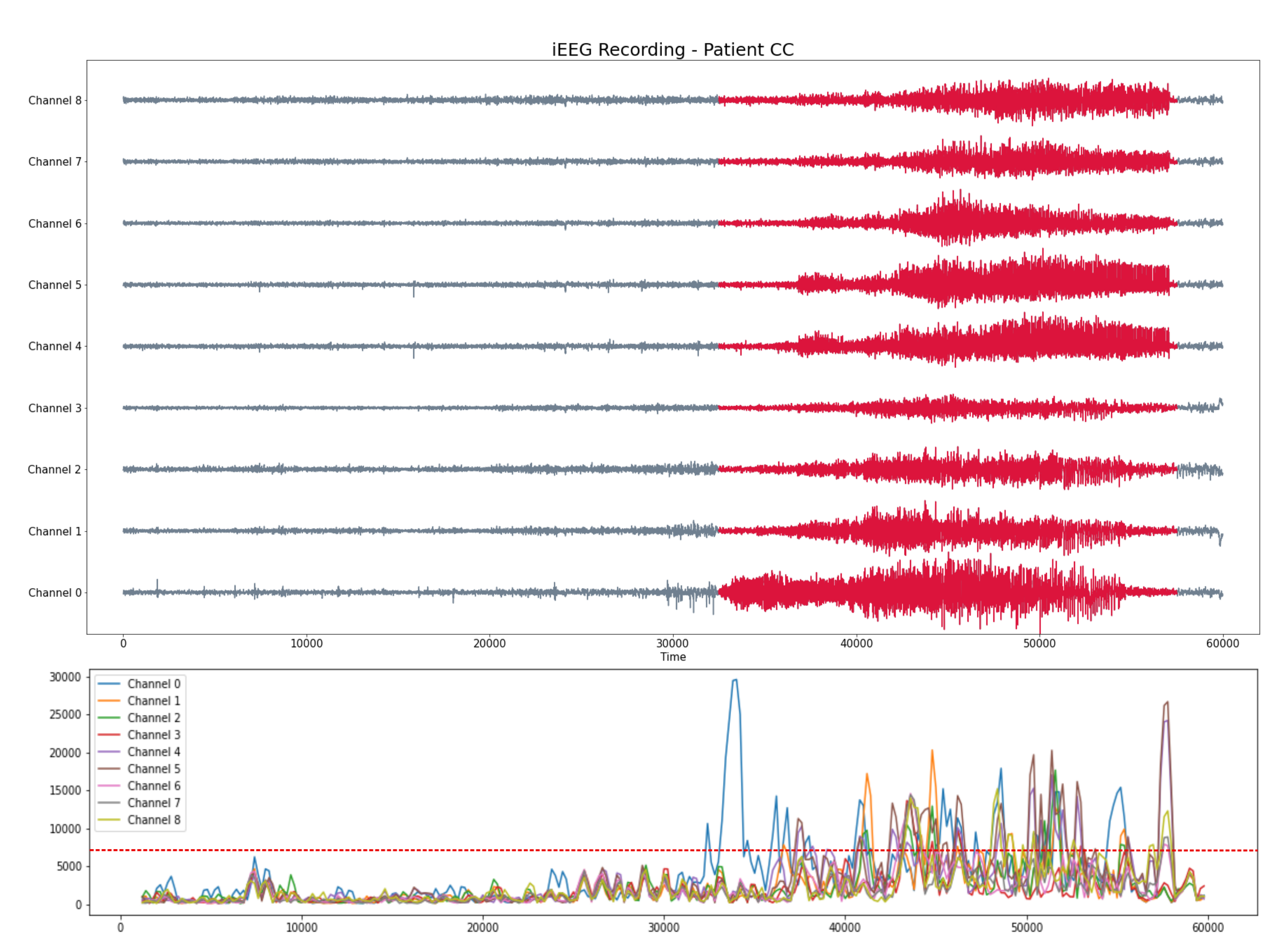
Patient CC
- iEEG with 9 channels
- 300 seg recording (baseline and seizure) with a sampling rate 200 HZ
Pacient CC
- iEEG with 9 channels
- 300 seg recording (baseline and seizure) with a sampling rate 200 HZ
- Seizure starts at $t = 32000$ and ends at $t =58000$
Pacient CC
- iEEG with 9 channels
- 300 seg recording (baseline and seizure) with a sampling rate 200 HZ
- Seizure starts at $t = 30000$ and ends at $t =58000$

Analysis by channel?
- Goal: Compare how local vs global dynamics changes over the time.
From single time series to topology
In theory, we assume we have a global continuous time dynamical system $(\mathcal{M}, \phi)$ with $\mathcal{M}$ a topological space and $\phi \colon \mathbb{R} \times \mathcal{M} \to \mathcal{M}$ a continuous map such that $\phi(0, p) = p$ and $\phi(s, \phi(𝑡, 𝑝)) = \phi(s + t, p)$ for all $p \in \mathcal{M}$ and all $t, s \in \mathbb{R}$.
In practice, we only have measurements that are the result of an observation function $F:X\to \mathbb R$ and an initial state $x_0\in X$ that produces a time series \begin{align}\varphi_p:\mathbb{R}&\to \mathbb{R}\\ t&\mapsto F(\phi_t(x_0)) \end{align}
We can topologically reconstruct the attractor from the observation.
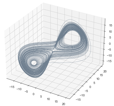
From time series to topology
In practice, we only have measurements that are the result of an observation function $F:X\to \mathbb R$ and an initial state $x_0\in X$ that produces a time series \begin{align}\varphi_{x_0}:\mathbb{R}&\to \mathbb{R}\\ t&\mapsto F(\phi_t(x_0)) \end{align}
Theorem (Takens). Let $\mathcal{M}$ be a smooth, compact, Riemannian manifold. Let $\tau > 0$ be a real number and let $d ≥ 2 \mathrm{dim}(\mathcal{M})$ be an integer. Then, for generic $\phi \in C^2(\mathbb{R} \times \mathcal{M}, \mathcal{M})$ and $F\in C^2(\mathcal{M}, \mathbb{R})$ and for $\varphi_\bullet(𝑡)$ defined as above, the delay map \begin{align} \varphi~ \colon & ~~\mathcal{M} &\rightarrow & ~~\mathbb{R}^{d+1}\\ &~~p &\mapsto & ~~(\varphi_p(0), \varphi_p(𝜏), \varphi_p(2𝜏),\dots, \varphi_p(d\tau)) \end{align} is an embedding (i.e., $\varphi$ is injective and its derivative has full-rank everywhere).
From time series to topology
The time delay embedding of $f$ with parameters $d$ and $\tau$ is the vector-valued function \begin{align} X_{d,\tau}f\colon &~~\mathbb{R}\rightarrow ~~\mathbb{R}^{d+1}\\ &~~~t ~\mapsto ~(f(t), 𝑓(t + \tau), 𝑓(t + 2\tau), \dots, 𝑓(t + d\tau))\\ \end{align}
Given time series data $f(t) = \varphi_p(t)$ with $t\in T$ observed from a potentially unknown dynamical system $(X, \phi)$, Takens’ theorem implies that (generically) the time delay embedding $X_{d,\tau}f([0,T])$ provides a topological copy of $\{\phi(t, x_0) ∶ t \in T\} \subseteq X$.
From time series to topology
The time delay embedding of $f$ with parameters $d$ and $\tau$ is the vector-valued function \begin{align} X_{d,\tau}f\colon &~~\mathbb{R}\rightarrow ~~\mathbb{R}^{d+1}\\ &~~~t ~\mapsto ~(f(t), 𝑓(t + \tau), 𝑓(t + 2\tau), \dots, 𝑓(t + d\tau))\\ \end{align}

Analysis by channel?
Channel $\to$ Sliding Window $\to$ Takens Delay Embedding $\to$ Path of persistent diagrams $\to$ 1st Derivative
Conclusions
- It is possible to topologically detect changes in the global dynamics by means of time-evolving persistent diagrams.
- Takens delay embedding provides a tool to (topologically) infer the global dynamic induced by a single observation.