Topological methods
for real-time detection of epileptic seizures
in EEG/MEG signals
XIMENA FERNANDEZ (joint work with Diego Mateos)
ximena.l.fernandez@durham.ac.uk
Durham University (UK), EPSRC Centre for Topological Data Analysis
DSABNS 2022 - February 8, 2022
The problem
- Data: Raw multichannel EEG/MEG recordings for different patients during preictal, ictal and interictal states.

The problem
- Data: Raw multichannel EEG/MEG recordings for different patients during preictal, ictal and interictal states.
- Goal: Detect the epileptic seizure.

Topological Time Series Analysis
Given $X_1, X_2, \dots X_N:[0,T]\to \mathbb{R}$ signals, we construct an embedding in $\mathbb{R}^N$ given by $$\{(X_1(t), X_2(t), \dots, X_N(t)): t\in [0,T]\}$$
Dynamical systems
We assume we are in the followig setting:
- A continuous dynamical system $(X, \phi)$, with $X$ a topological space and $\phi_t \colon X \to X$ a smooth family of evolution functions for $t \in \mathbb{R}$.
- A set $A \subset X$ called the attractor, that is the asymptotic state of the system.
Dynamical systems
- A continuous dynamical system $(X, \phi)$, with $X$ a topological space and $\phi_t \colon X \to X$ a smooth family of evolution functions for $t \in \mathbb{R}$.
- A set $A \subset X$ called the attractor, that is the asymptotic state of the system.
- The typical examples arising from differential equations have as state space a smooth manifold $X$ and the dynamics are given by the integral curves of a smooth vector field on $X$.
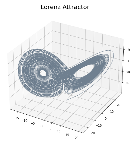
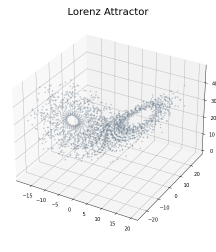
Lorenz attractor \begin{equation}\begin{cases} \dot x = \sigma ( y - x ) , \\ \dot y = x(\rho-z)-y ,\\ \dot z = xy-\beta z \end{cases} \end{equation} with $(\sigma, \rho, \beta) = (10, 28, 8/3)$.
Dynamical systems
- A continuous dynamical system $(X, \phi)$, with $X$ is a topological space and $\phi_t \colon X \to X$ a smooth family of evolution functions for $t \in \mathbb{R}$.
- A set $A \subset X$ called the attractor, that is the asymptotic state of the system.
Geometry of the attractor
- Given a topological space $X$, its homology $H_k(X)$ at degree $k$ captures geometric signatures in $X$ of dimension $k$.
- The rank of the group $H_k(X)$ defines the $k$-th Betti number $\beta_k$ of $X$ and it quantifies the number of (independent) $k$-dimensional holes in $X$.
- $\beta_0$ = number of connected components,
- $\beta_1$ = number of 1-dimensional cycles,
- $\beta_2$ = number of 2-dimensional voids, $\dots$
- $\beta_0$ = 1
- $\beta_1$ = 2
- $\beta_2$ = 0
Geometry of the attractor
- Given a topological space $X$, its homology $H_k(X)$ at degree $k$ captures geometric signatures in $X$ of dimension $k$.
- The rank of the group $H_k(X)$ defines the $k$-th Betti number $\beta_k$ of $M$ and it quantifies the number of (independent) $k$-dimensional holes in $M$.
- $\beta_0$ = number of connected components,
- $\beta_1$ = number of 1-dimensional cycles,
- $\beta_2$ = number of 2-dimensional voids, $\dots$
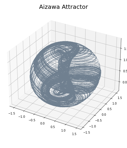
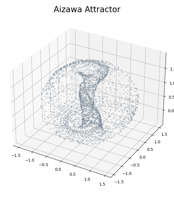
- $\beta_0$ = 1
- $\beta_1$ = 1
- $\beta_2$ = 1
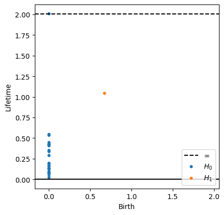
Geometry of a sample of the attractor
- Given a sample $X_n$ of a topological space, its persistent homology at degree $k$ infers geometric signatures of dimension $k$ in the underlying space.
Point cloud

Geometry of a sample of the attractor
- Given a sample $X_n$ of a topological space, its persistent homology at degree $k$ infers geometric signatures of dimension $k$ in the underlying space.
- The computation relies in the reconstruction of the underlying space as union of balls centered in the sample points with increasing radii.
Point cloud
Filtration of spaces

Geometry of a sample of the attractor
- Given a sample $X_n$ of a topological space, its persistent homology at degree $k$ infers geometric signatures of dimension $k$ in the underlying space.
- The computation relies in the reconstruction of the underlying space as union of balls centered in the sample points with increasing radii.
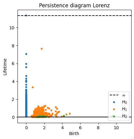
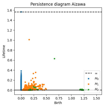
- The persistence diagram at degree $k$ has a point for each generator in $H_k$ in the filtration, the 1st coordinate represents its birth, the 2nd coordinate represents its lifetime.
Point cloud
Filtration of spaces
Persistence diagram
Geometry of a sample of the attractor
- Given a sample $X_n$ of a topological space, its persistent homology at degree $k$ infers geometric signatures of dimension $k$ in the underlying space.
- The computation relies in the reconstruction of the underlying space as union of balls centered in the sample points with increasing radii.
- The persistence diagram at degree $k$ has a point for each generator in $H_k$ in the filtration, the 1st coordinate represents its birth, the 2nd coordinate represents its lifetime.
Sliding Window Embedding
- Let $X_1, X_2, \dots X_N:[0,T]\to \mathbb{R}$ a set of signals.
- Given a window size $W$, we compute for every $t\in [W,T]$ the embedding of $X_1, X_2, \dots X_N:[t-W, t]\to \mathbb{R}$ in $\mathbb{R}^N$.
Sliding Window Embedding
- Let $X_1, X_2, \dots X_N:[0,T]\to \mathbb{R}$ a set of signals.
- Given a window size $W$, we compute for every $t\in [W,T]$ the embedding of $X_1, X_2, \dots X_N:[t-W, t]\to \mathbb{R}$ in $\mathbb{R}^N$.
Sliding Window Embedding
- Let $X_1, X_2, \dots X_N:[0,T]\to \mathbb{R}$ a set of signals.
- Given a window size $W$, we compute for every $t\in [W,T]$ the embedding of $X_1, X_2, \dots X_N:[t-W, t]\to \mathbb{R}$ in $\mathbb{R}^N$.
- We compute the (persistent) homology of the time evolving sliding window embedding.

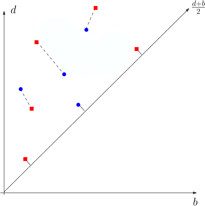
Metric in the space of persistence diagrams
- The Wassertein distance between two diagrams $\mathrm{dgm}_1$ and $\mathrm{dgm}_2$ is \[d_W(\mathrm{dgm}_1, \mathrm{dgm}_2) = \inf_{M \text{ matching}} \left(\sum_{(x,y)\in M} ||x-y||^p\right)^{1/p}\]
Real time detection of epileptic seizures
in EEG/MEG recordings
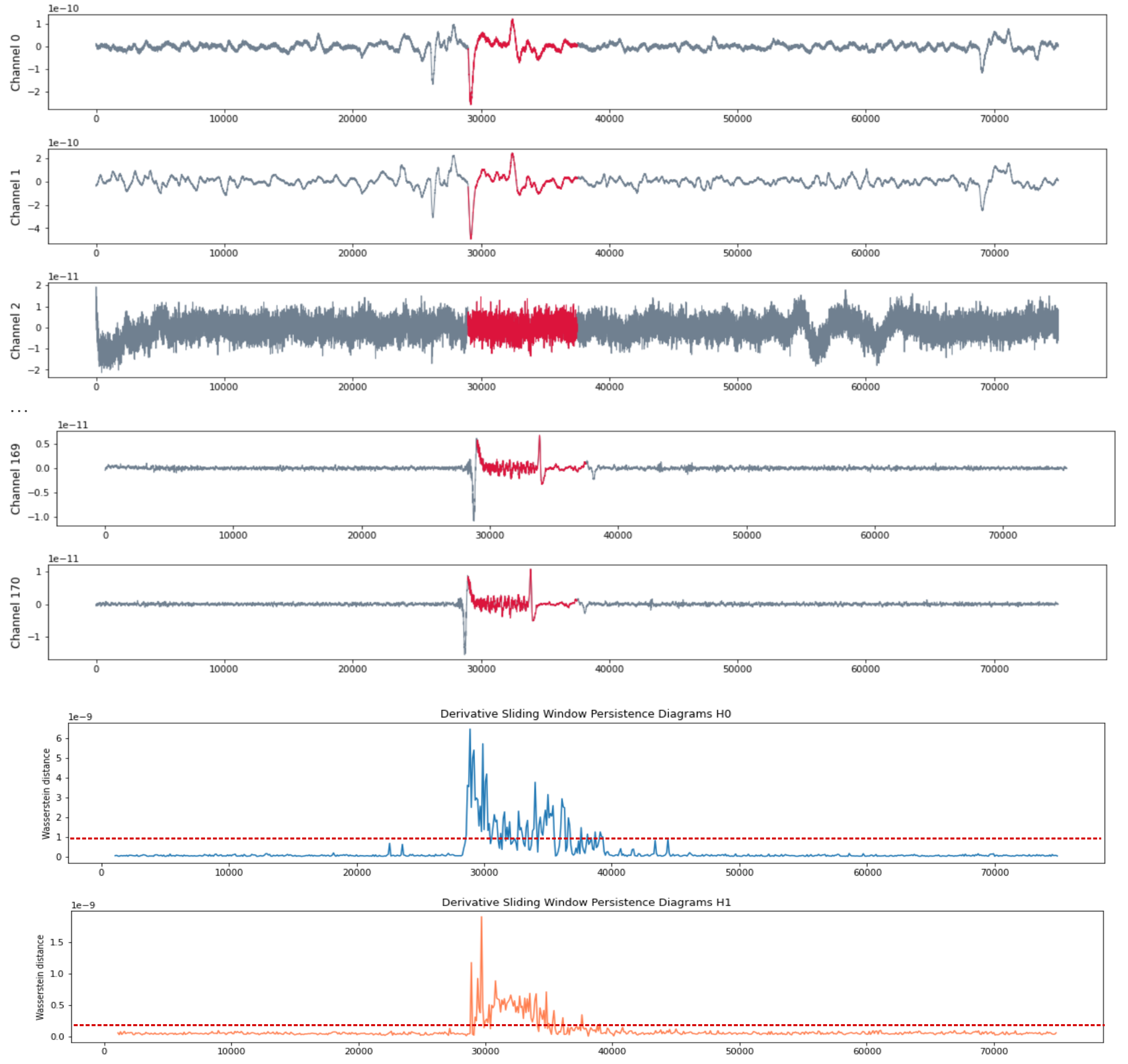
Multichannel signals $\to$ Sliding Window Embedding $\to$ Path of persistent diagrams $\to$ (Estimator of) 1st Derivative

Experiments
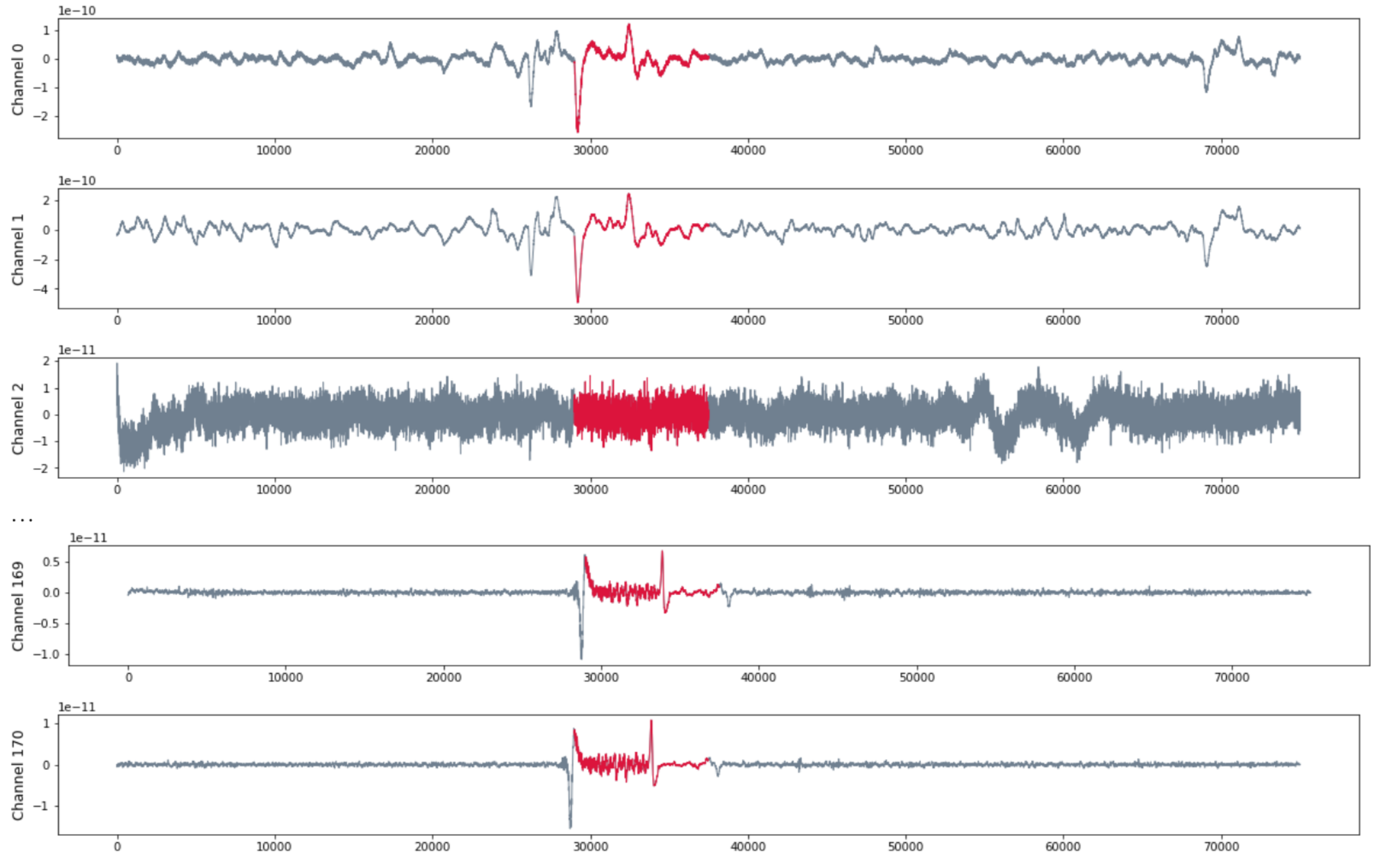
Patient RAO
- MEG with 171 channels
- 120 seg recording with sampling rate 625 HZ

Patient RAO
- MEG with 171 channels
- 120 seg recording with sampling rate 625 HZ
- Seizure starts at $t = 29375$ and ends at $t = 37500$.
Patient RAO
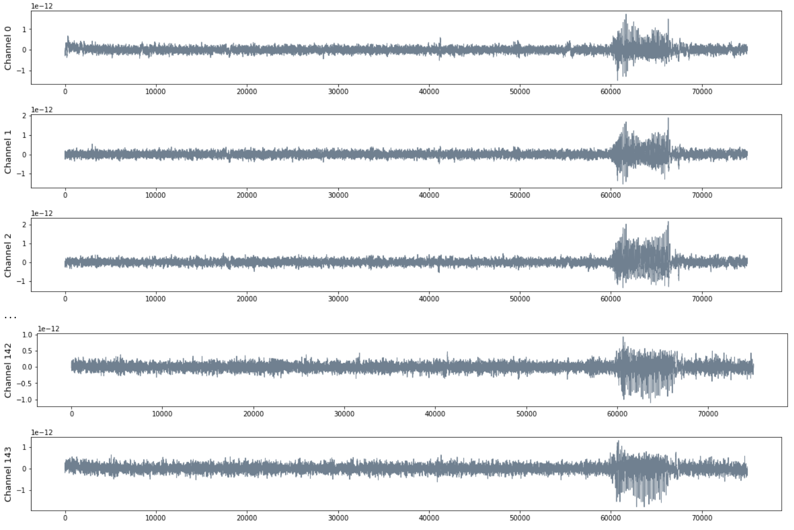
Patient MAC
- MEG with 144 channels
- 120 seg recording with sampling rate 625 HZ
Patient MAC
- MEG with 144 channels
- 120 seg recording with sampling rate 625 HZ
- Seizure starts at $t = 60000$ and ends at $t = 68125$.
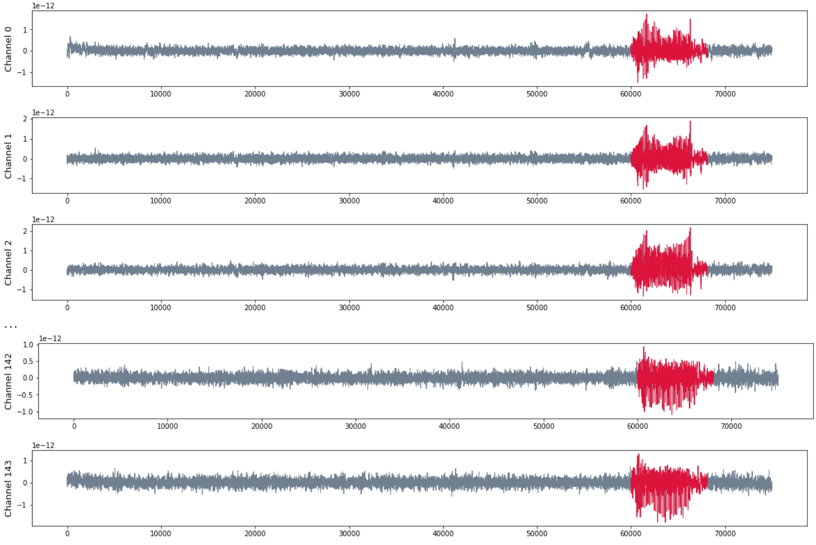
Patient MAC
- MEG with 144 channels
- 120 seg recording with sampling rate 625 HZ
- Seizure starts at $t = 60000$ and ends at $t = 68125$.

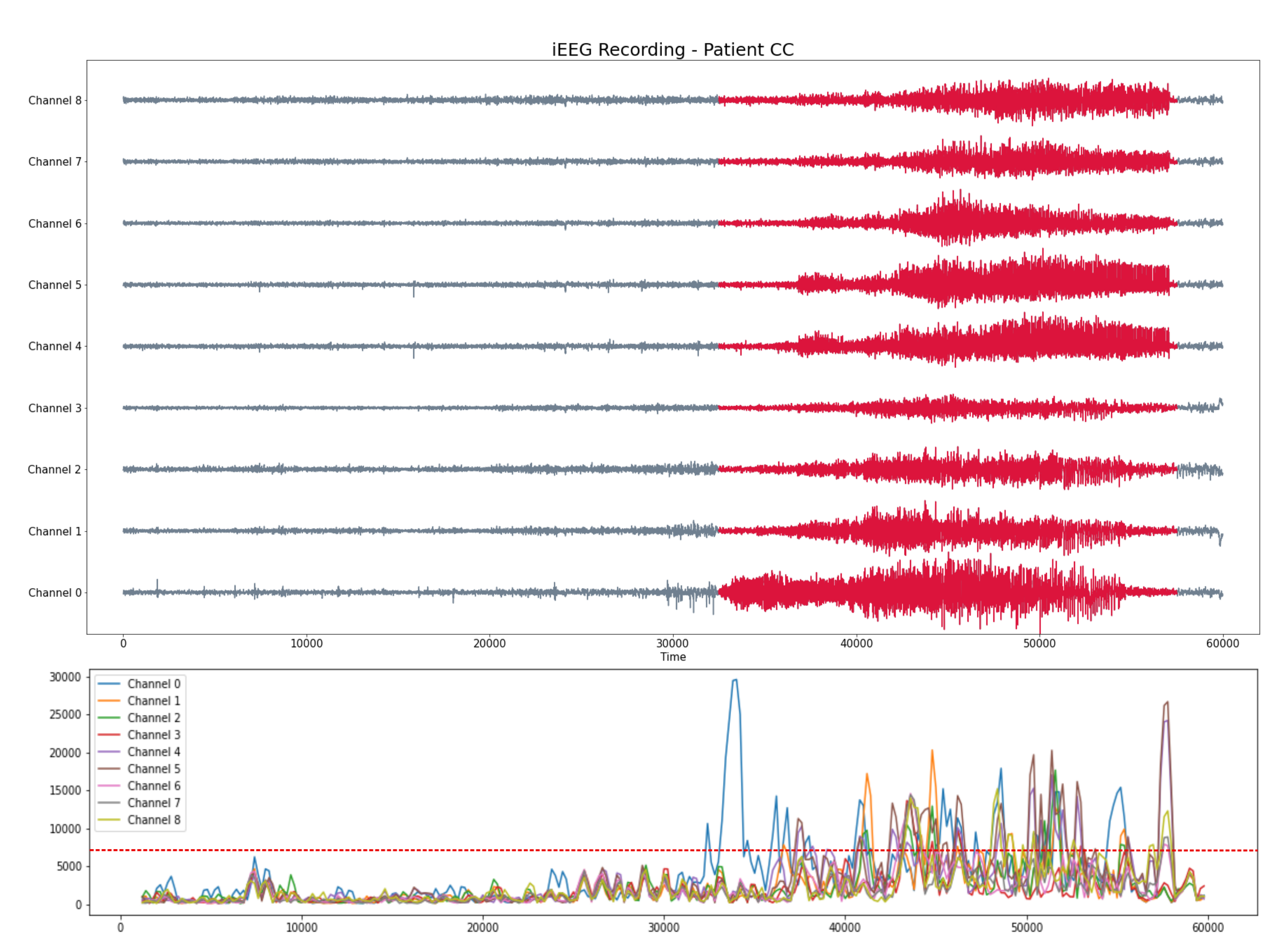
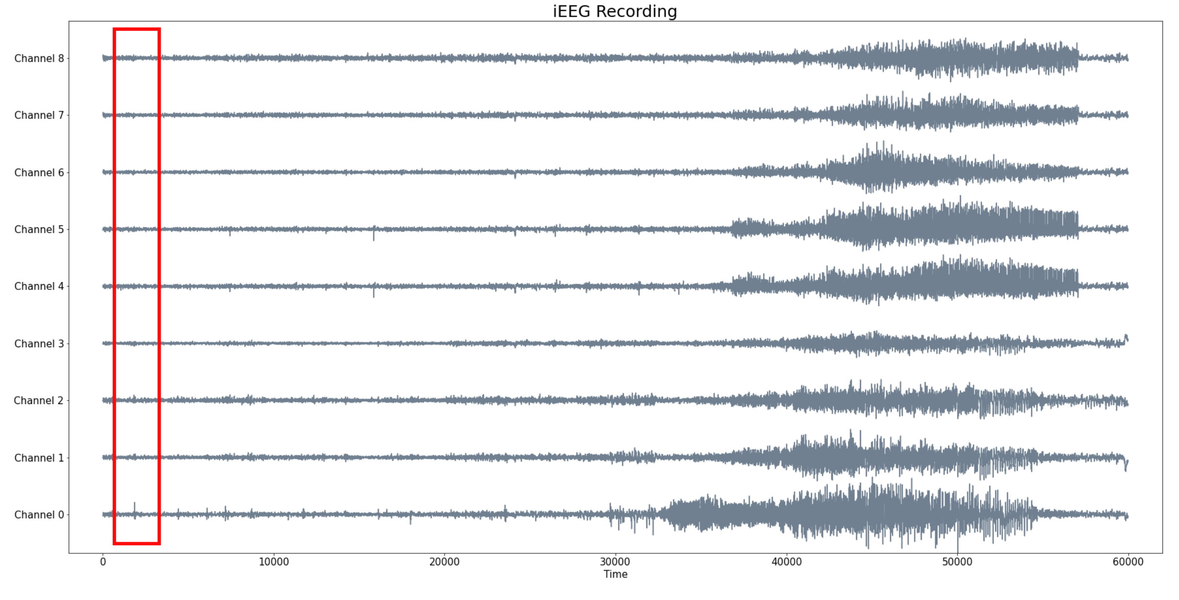
Patient CC
- iEEG with 9 channels
- 300 seg recording (baseline and seizure) with a sampling rate 200 HZ
Pacient CC
- iEEG with 9 channels
- 300 seg recording (baseline and seizure) with a sampling rate 200 HZ
- Seizure starts at $t = 30000$ and ends at $t =58000$
Pacient CC
- iEEG with 9 channels
- 300 seg recording (baseline and seizure) with a sampling rate 200 HZ
- Seizure starts at $t = 30000$ and ends at $t =58000$

Bonus: analysis by channel
- For every channel $X_i:[0,T]\colon \rightarrow \mathbb{R}$, compute the dynamic induced by this observation.
- Compare the induced maps of time evolving topological changes, for the different channels.
Bonus: analysis by channel
- For every channel $X_i:[0,T]\colon \rightarrow \mathbb{R}$, compute the dynamic induced by this observation.
Given a signal $X:[0,T] \to \mathbb{R}$, the delay embedding in dimension $d$ and delay $\tau$ is \[\{(X(t), X(t+\tau), X(t+2\tau), \dots, X(t+(d-1)\tau)\in \mathbb{R}^d: t\in[0, T-(d-1)\tau]\}\]
Takens Theorem. The delay embedding of an observation allows to reconstruct the entire dynamics.

Bonus: analysis by channel
Channel $\to$ Sliding Window Delay Embedding $\to$ Path of persistent diagrams $\to$ 1st Derivative